Convection Diffusion 2D Example on Circular Domain

This example demonstrates how to solve a Poisson equation in 2D on a circular domain using the fastvpinns package. All the necessary files can be found in the examples folder of the fastvpinns GitHub repository

The Poisson equation is given by

\[-\varepsilon \nabla^2 u + \mathbf{b} \cdot \nabla u + cu = f \quad \text{in} \quad \Omega\]

where \(\Omega\) is the circular domain and \(f\) is the source term. The boundary conditions are given by

\[u = \cos(x^2 + y^2) \quad \text{on} \quad \partial \Omega\]

For this problem, the parameters are

\[ \begin{align}\begin{aligned}f = 4x^2\cos(x^2 + y^2) - 2x\sin(x^2 + y^2) + 4y^2\cos(x^2 + y^2) + 4\sin(x^2 + y^2)\\\varepsilon = 1, \mathbf{b} = [1, 0], c = 0\end{aligned}\end{align} \]

The exact solution is given by

\[u = cos(x^2 +y^2)\]

Note : The forcing formulation for this problem is obtained by substituting the exact solution into the cd2d equation with given pde parameters.

Computational Domain

The computational domain is a circular domain with radius 1 centered at (0, 0).

Contents

• Steps to run the code

• Example File

  • Defining the boundary conditions

  • Defining the source term

  • Defining the exact solution

  • Defining the bilinear form

• Input File

  • Experimentation parameters

  • Geometry parameters

  • Finite element space parameters

  • PDE Beta parameters

  • Model parameters

  • Logging parameters

• Main File

  • Importing the required libraries

  • Imports from fastvpinns

  • Reading the input file

  • Reading all input parameters

  • Setup the geometry

  • Setup fespace

  • Setup datahandler

  • Setup model

  • Pre-train setup

  • Training

  • Post Training

• Save the outputs

• Solution Plots

• References

Steps to run the code

To run the code, execute the following command:

python3 main_cd2d.py input.yaml

Back to Contents

Example File

The example file cd2d_example.py, hosts all the details about the bilinear parameters for the PDE, boundary conditions, source term, and the exact solution.

Back to Contents

Defining the boundary conditions

The function circle_boundary returns the boundary value for a given component of the boundary. The function get_boundary_function_dict returns a dictionary of boundary functions. The key of the dictionary is the boundary id and the value is the boundary function. The function get_bound_cond_dict returns a dictionary of boundary conditions.

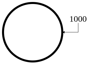
For externally created geometries from gmsh, the user needs to provide the physical tag for the boundaries present in the geometry. In our case, we have used 1000 to define the circular boundary in mesh file.

Note : As of now, only Dirichlet boundary conditions are supported.

def circle_boundary(x, y):
    """
    This function will return the boundary value for given component of a boundary
    """
    return 0.0

def get_boundary_function_dict():
    """
    This function will return a dictionary of boundary functions
    """
    return {1000: circle_boundary}


def get_bound_cond_dict():
    """
    This function will return a dictionary of boundary conditions
    """
    return {1000: "dirichlet"}

Back to Contents

Defining the source term

The function rhs returns the value of the source term at a given point.

def rhs(x, y):
    """
    This function will return the value of the rhs at a given point
    """
    f_temp = 32 * (x * (1 - x) + y * (1 - y))

    return f_temp

Back to Contents

Defining the exact solution

The function exact_solution returns the value of the exact solution at a given point.

def exact_solution(x, y):
    """
    This function will return the value of the exact solution at a given point
    """
    u_temp = 16 * x * (1 - x) * y * (1 - y)

    return u_temp

Back to Contents

Defining the bilinear form

The function get_bilinear_params_dict returns a dictionary of bilinear parameters. The dictionary contains the values of the parameters \(\varepsilon\) (varepsilon), \(b_x\) (convection in x-direction), \(b_y\) (convection in y-direction), and \(c\) (reaction term).

Note : If any of the bilinear parameters are not present in the dictionary (for the cd2d model), then the code will throw an error.

def get_bilinear_params_dict():
    """
    This function will return a dictionary of bilinear parameters
    """
    eps = 1.0
    b_x = 1.0
    b_y = 0.0
    c = 0.0

    return {"eps": eps, "b_x": b_x, "b_y": b_y, "c": c}

Back to Contents

Input File

This file contains all the details about the problem. The input file is in the YAML format. The input file for this example is given below. The contents of the yaml files are as follows

Back to Contents

Experimentation parameters

Defines the output path where the results will be saved.

experimentation:
  output_path: "output/cd2d/1"  # Path to the output directory where the results will be saved.

Back to Contents

Geometry parameters

It contains the details about the geometry of the domain. The mesh generation method can be either “internal” or “external”. If the mesh generation method is “internal”, then the internal_mesh_params are used to generate the mesh. If the mesh generation method is “external”, then the mesh is read from the file specified in the mesh_file parameter.

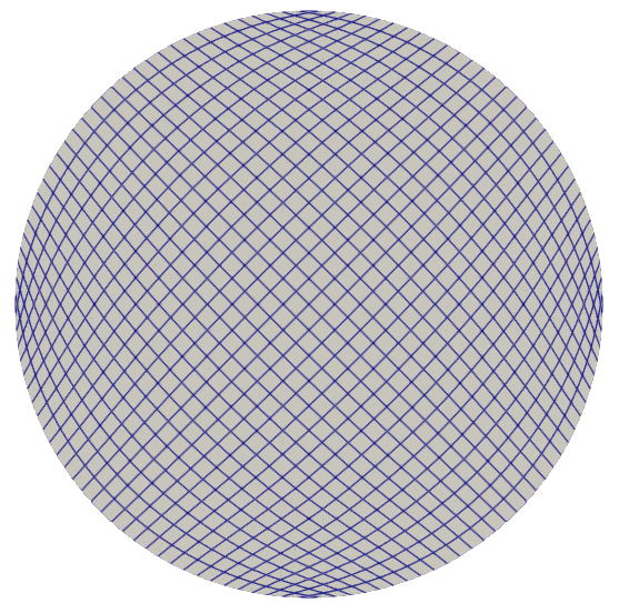
• In this case, we will use an external mesh. The mesh ../meshes/circle_quad.mesh is generated using the Gmsh software. The mesh needs to have physical elements defined for the boundary. In this case, the physical element is defined as 1000 (which is defined in the circle_boundary function in the cd2d_example.py file).

• exact_solution_generation is set to “internal” which means that the exact solution is generated using the exact_solution function in the cd2d_example.py file.

• mesh_type is set to “quadrilateral” which means that the mesh is a quadrilateral mesh. Note: As of now, only quadrilateral meshes are supported.

• boundary_refinement_level is set to 4 which means that the boundary is refined 4 times. (i.e), when the mesh is read, only the boundary points of an edge in quadrilateral mesh are read. this refinement will refine the boundary points to get more boundary points within the edge.

• boundary_sampling_method is set to “uniform” which means that the boundary points are sampled using the “uniform” method. (Use only uniform sampling as of now.)

• generate_mesh_plot is set to True which means that the mesh plot is generated and saved in the output directory.

geometry:
  mesh_generation_method: "external"  # Method for generating the mesh. Can be "internal" or "external".
  generate_mesh_plot: True  # Flag indicating whether to generate a plot of the mesh.

  # internal mesh generated quadrilateral mesh, depending on the parameters specified below.

  internal_mesh_params:  # Parameters for internal mesh generation method.
    x_min: 0  # Minimum x-coordinate of the domain.
    x_max: 1  # Maximum x-coordinate of the domain.
    y_min: 0  # Minimum y-coordinate of the domain.
    y_max: 1  # Maximum y-coordinate of the domain.
    n_cells_x: 4  # Number of cells in the x-direction.
    n_cells_y: 4  # Number of cells in the y-direction.
    n_boundary_points: 400  # Number of boundary points.
    n_test_points_x: 100  # Number of test points in the x-direction.
    n_test_points_y: 100  # Number of test points in the y-direction.

  exact_solution:
    exact_solution_generation: "internal" # whether the exact solution needs to be read from external file.
    exact_solution_file_name: "" # External solution file name.

  mesh_type: "quadrilateral"  # Type of mesh. Can be "quadrilateral" or other supported types.

  external_mesh_params:  # Parameters for external mesh generation method.
    mesh_file_name: "../meshes/circle_quad.mesh"  # Path to the external mesh file (should be a .mesh file).
    boundary_refinement_level: 4  # Level of refinement for the boundary.
    boundary_sampling_method: "lhs"  # Method for sampling the boundary. Can be "uniform" or "lhs".

Back to Contents

Finite Element Space parameters

This section contains the details about the finite element spaces.

fe:
  fe_order: 6 # Order of the finite element basis functions.
  fe_type: "legendre"  # Type of finite element basis functions. Can be "jacobi" or other supported types.
  quad_order: 10  # Order of the quadrature rule.
  quad_type: "gauss-jacobi"

Here the fe_order is set to 6 which means it has 6 basis functions in each direction. The quad_order is set to 10 which means it uses a 10-points in each direction for the quadrature rule. The supported quadrature rules are “gauss-jacobi” and “gauss-legendre”. In this version of code, both “jacobi” and “legendre” refer to the same basis functions (to maintain backward compatibility). The basis functions are special type of Jacobi polynomials defined by

\[J_{n} = J_{n-1} - J_{n+1}\]

, where J _n is the nth Jacobi polynomial.

Back to Contents

PDE beta parameters

This value provides the beta values for the Dirichlet boundary conditions. The beta values are the multipliers that are used to multiply the boundary losses.

\[loss_{total} = loss_{pde} + \beta \cdot loss_{dirichlet}\]

pde:
  beta: 10  # Parameter for the PDE.

Back to Contents

Model parameters

The model section contains the details about the dense model to be used.

• The model architecture is given by the model_architecture parameter.

• The activation function used in the model is given by the activation parameter.

• The epochs parameter is the number of training epochs.

• The dtype parameter is the data type used for computations.

• The learning_rate section contains the parameters for learning rate scheduling.

• The initial_learning_rate parameter is the initial learning rate.

• The use_lr_scheduler parameter is a flag indicating whether to use the learning rate scheduler.

• The decay_steps parameter is the number of steps between each learning rate decay.

• The decay_rate parameter is the decay rate for the learning rate.

• The staircase parameter is a flag indicating whether to use the staircase decay.

Any parameter which are not mentioned above are archived parameters, which are not used in the current version of the code. (like use_attention, set_memory_growth)

model:
  model_architecture: [2, 50,50,50,50, 1]  # Architecture of the neural network model.
  activation: "tanh"  # Activation function used in the neural network.
  use_attention: False  # Flag indicating whether to use attention mechanism in the model.
  epochs: 50000  # Number of training epochs.
  dtype: "float32"  # Data type used for computations.
  set_memory_growth: False  # Flag indicating whether to set memory growth for GPU.

  learning_rate:  # Parameters for learning rate scheduling.
    initial_learning_rate: 0.001  # Initial learning rate.
    use_lr_scheduler: False  # Flag indicating whether to use learning rate scheduler.
    decay_steps: 1000  # Number of steps between each learning rate decay.
    decay_rate: 0.99  # Decay rate for the learning rate.
    staircase: False

Back to Contents

Logging parameters

update_console_output defines the epochs at which you need to log parameters like loss, time taken, etc.

logging:
  update_console_output: 100  # Number of epochs after which to update the console output.

The other parameters such as update_progress_bar, update_solution_images are archived parameters which are not used in the current version of the code.

Back to Contents

Main File

The file main_cd2d.py contains the main code to solve the Poisson equation in 2D on a circular domain. The code reads the input file, sets up the problem, and solves the Poisson equation using the fastvpinns package.

Back to Contents

Importing the required libraries

The following libraries are imported in the main file.

import numpy as np
import pandas as pd
import pytest
import tensorflow as tf
from pathlib import Path
from tqdm import tqdm
import yaml
import sys
import copy
from tensorflow.keras import layers
from tensorflow.keras import initializers
from rich.console import Console
import copy
import time

Back to Contents

Imports from fastvpinns

The following imports are used from the fastvpinns package.

• Imports the geometry module from the fastvpinns package, which contains the Geometry_2D class responsible for setting up the geometry of the domain.

from fastvpinns.Geometry.geometry_2d import Geometry_2D

• Imports the fespace module from the fastvpinns package, which contains the FE class responsible for setting up the finite element spaces.

from fastvpinns.FE.fespace2d import Fespace2D

• Imports the datahandler module from the fastvpinns package, which contains the DataHandler class responsible for handling and converting the data to necessary shape for training purposes

from fastvpinns.DataHandler.datahandler import DataHandler

• Imports the model module from the fastvpinns package, which contains the Model class responsible for training the neural network model.

from fastvpinns.Model.model import DenseModel

• Import the Loss module from the fastvpinns package, which contains the loss function of the PDE to be solved in tensor form.

from fastvpinns.physics.cd2d import pde_loss_cd2d

• Import additional functionalities from the fastvpinns package.

from fastvpinns.utils.plot_utils import plot_contour, plot_loss_function, plot_test_loss_function
from fastvpinns.utils.compute_utils import compute_errors_combined
from fastvpinns.utils.print_utils import print_table

Back to Contents

Reading the input file

The input file is read using the yaml library.

if len(sys.argv) != 2:
        print("Usage: python main.py <input file>")
        sys.exit(1)

    # Read the YAML file
    with open(sys.argv[1], 'r') as f:
        config = yaml.safe_load(f)

Back to Contents

Reading all input parameters

# Extract the values from the YAML file
    i_output_path = config['experimentation']['output_path']

    i_mesh_generation_method = config['geometry']['mesh_generation_method']
    i_generate_mesh_plot = config['geometry']['generate_mesh_plot']
    i_mesh_type = config['geometry']['mesh_type']
    i_x_min = config['geometry']['internal_mesh_params']['x_min']
    i_x_max = config['geometry']['internal_mesh_params']['x_max']
    i_y_min = config['geometry']['internal_mesh_params']['y_min']
    i_y_max = config['geometry']['internal_mesh_params']['y_max']
    i_n_cells_x = config['geometry']['internal_mesh_params']['n_cells_x']
    i_n_cells_y = config['geometry']['internal_mesh_params']['n_cells_y']
    i_n_boundary_points = config['geometry']['internal_mesh_params']['n_boundary_points']
    i_n_test_points_x = config['geometry']['internal_mesh_params']['n_test_points_x']
    i_n_test_points_y = config['geometry']['internal_mesh_params']['n_test_points_y']
    i_exact_solution_generation = config['geometry']['exact_solution']['exact_solution_generation']
    i_exact_solution_file_name = config['geometry']['exact_solution']['exact_solution_file_name']

    i_mesh_file_name = config['geometry']['external_mesh_params']['mesh_file_name']
    i_boundary_refinement_level = config['geometry']['external_mesh_params'][
        'boundary_refinement_level'
    ]
    i_boundary_sampling_method = config['geometry']['external_mesh_params'][
        'boundary_sampling_method'
    ]

    i_fe_order = config['fe']['fe_order']
    i_fe_type = config['fe']['fe_type']
    i_quad_order = config['fe']['quad_order']
    i_quad_type = config['fe']['quad_type']

    i_model_architecture = config['model']['model_architecture']
    i_activation = config['model']['activation']
    i_use_attention = config['model']['use_attention']
    i_epochs = config['model']['epochs']
    i_dtype = config['model']['dtype']
    if i_dtype == "float64":
        i_dtype = tf.float64
    elif i_dtype == "float32":
        i_dtype = tf.float32
    else:
        print("[ERROR] The given dtype is not a valid tensorflow dtype")
        raise ValueError("The given dtype is not a valid tensorflow dtype")

    i_set_memory_growth = config['model']['set_memory_growth']
    i_learning_rate_dict = config['model']['learning_rate']

    i_beta = config['pde']['beta']

    i_update_console_output = config['logging']['update_console_output']

All the variables which are named with the prefix i_ are input parameters which are read from the input file.

Back to Contents

Setup the geometry

Obtain the boundary condition and boundary values from the cd2d_example.py file and initialise the Geometry_2D class. After that use the domain.read_mesh functionality to read the external mesh file.

cells, boundary_points = domain.read_mesh(
        i_mesh_file_name,
        i_boundary_refinement_level,
        i_boundary_sampling_method,
        refinement_level=1,
    )

Back to Contents

Setup fespace

Initialise the Fespace2D class with the required parameters.

fespace = Fespace2D(
        mesh=domain.mesh,
        cells=cells,
        boundary_points=boundary_points,
        cell_type=domain.mesh_type,
        fe_order=i_fe_order,
        fe_type=i_fe_type,
        quad_order=i_quad_order,
        quad_type=i_quad_type,
        fe_transformation_type="bilinear",
        bound_function_dict=bound_function_dict,
        bound_condition_dict=bound_condition_dict,
        forcing_function=rhs,
        output_path=i_output_path,
        generate_mesh_plot=i_generate_mesh_plot,
    )

Back to Contents

Setup datahandler

Initialise the DataHandler class with the required parameters.

datahandler = DataHandler2D(fespace, domain, dtype=i_dtype)

Back to Contents

Setup model

Setup the necessary parameters for the model and initialise the Model class. Before that fill the params dictionary with the required parameters.

model = DenseModel(
        layer_dims=[2, 30, 30, 30, 1],
        learning_rate_dict=i_learning_rate_dict,
        params_dict=params_dict,
        loss_function=pde_loss_cd2d,
        input_tensors_list=[datahandler.x_pde_list, train_dirichlet_input, train_dirichlet_output],
        orig_factor_matrices=[
            datahandler.shape_val_mat_list,
            datahandler.grad_x_mat_list,
            datahandler.grad_y_mat_list,
        ],
        force_function_list=datahandler.forcing_function_list,
        tensor_dtype=i_dtype,
        use_attention=i_use_attention,
        activation=i_activation,
        hessian=False,
    )

Back to Contents

Pre-train setup

test_points = domain.get_test_points()
  print(f"[bold]Number of Test Points = [/bold] {test_points.shape[0]}")
  y_exact = exact_solution(test_points[:, 0], test_points[:, 1])

  # plot the exact solution
  num_epochs = i_epochs  # num_epochs
  progress_bar = tqdm(
      total=num_epochs,
      desc='Training',
      unit='epoch',
      bar_format="{l_bar}{bar:40}{r_bar}{bar:-10b}",
      colour="green",
      ncols=100,
  )
  loss_array = []  # total loss
  test_loss_array = []  # test loss
  time_array = []  # time per epoc
  # beta - boundary loss parameters
  beta = tf.constant(i_beta, dtype=i_dtype)

This sets up the test points and the exact solution. The progress bar is initialised and the loss arrays are set up. The beta value is set up as a constant tensor.

Back to Contents

Training

for epoch in range(num_epochs):

    # Train the model
    batch_start_time = time.time()
    loss = model.train_step(beta=beta, bilinear_params_dict=bilinear_params_dict)
    elapsed = time.time() - batch_start_time

    # print(elapsed)
    time_array.append(elapsed)

    loss_array.append(loss['loss'])

This train_step function trains the model for one epoch and returns the loss. The loss is appended to the loss array. Then for every epoch where (epoch + 1) % i_update_console_output == 0 or epoch == num_epochs - 1:

y_pred = model(test_points).numpy()
y_pred = y_pred.reshape(-1)

error = np.abs(y_exact - y_pred)

# get errors
(
    l2_error,
    linf_error,
    l2_error_relative,
    linf_error_relative,
    l1_error,
    l1_error_relative,
) = compute_errors_combined(y_exact, y_pred)

loss_pde = float(loss['loss_pde'].numpy())
loss_dirichlet = float(loss['loss_dirichlet'].numpy())
total_loss = float(loss['loss'].numpy())

# Append test loss
test_loss_array.append(l1_error)

solution_array = np.c_[y_pred, y_exact, np.abs(y_exact - y_pred)]
domain.write_vtk(
    solution_array,
    output_path=i_output_path,
    filename=f"prediction_{epoch+1}.vtk",
    data_names=["Sol", "Exact", "Error"],
)

console.print(f"\nEpoch [bold]{epoch+1}/{num_epochs}[/bold]")
console.print("[bold]--------------------[/bold]")
console.print("[bold]Beta : [/bold]", beta.numpy(), end=" ")
console.print(
    f"Variational Losses || Pde Loss : [red]{loss_pde:.3e}[/red] Dirichlet Loss : [red]{loss_dirichlet:.3e}[/red] Total Loss : [red]{total_loss:.3e}[/red]"
)
console.print(
    f"Test Losses        || L1 Error : {l1_error:.3e} L2 Error : {l2_error:.3e} Linf Error : {linf_error:.3e}"
)

We will compute all the test errors and write the solution to a vtk file for a complex mesh. Further, the console output will be printed with the loss values and the test errors.

Back to Contents

Post Training

# Save the model
  model.save_weights(str(Path(i_output_path) / "model_weights"))

  solution_array = np.c_[y_pred, y_exact, np.abs(y_exact - y_pred)]
  domain.write_vtk(
      solution_array,
      output_path=i_output_path,
      filename=f"prediction_{epoch+1}.vtk",
      data_names=["Sol", "Exact", "Error"],
  )
  # print the Error values in table
  print_table(
      "Error Values",
      ["Error Type", "Value"],
      [
          "L2 Error",
          "Linf Error",
          "Relative L2 Error",
          "Relative Linf Error",
          "L1 Error",
          "Relative L1 Error",
      ],
      [l2_error, linf_error, l2_error_relative, linf_error_relative, l1_error, l1_error_relative],
  )

  # print the time values in table
  print_table(
      "Time Values",
      ["Time Type", "Value"],
      [
          "Time per Epoch(s) - Median",
          "Time per Epoch(s) IQR-25% ",
          "Time per Epoch(s) IQR-75% ",
          "Mean (s)",
          "Epochs per second",
          "Total Train Time",
      ],
      [
          np.median(time_array),
          np.percentile(time_array, 25),
          np.percentile(time_array, 75),
          np.mean(time_array),
          int(i_epochs / np.sum(time_array)),
          np.sum(time_array),
      ],
  )

  # save all the arrays as numpy arrays
  np.savetxt(str(Path(i_output_path) / "loss_function.txt"), np.array(loss_array))
  np.savetxt(str(Path(i_output_path) / "prediction.txt"), y_pred)
  np.savetxt(str(Path(i_output_path) / "exact.txt"), y_exact)
  np.savetxt(str(Path(i_output_path) / "error.txt"), error)
  np.savetxt(str(Path(i_output_path) / "time_per_epoch.txt"), np.array(time_array))

This part of the code saves the model weights, writes the solution to a vtk file, prints the error values in a table, prints the time values in a table, and saves all the arrays as numpy arrays.

Back to Contents

Save the outputs

All the outputs will be saved in the output directory specified in the input file. The output directory will contain the following files:

• prediction_{epoch}.vtk : The solution file for each epoch.

• loss_function.txt : The loss function values for each epoch.

• prediction.txt : The predicted values at last epoch at the test points.

• exact.txt : The exact values at last epoch at the test points.

• error.txt : The error values at last epoch at the test points.

• time_per_epoch.txt : The time taken for each epoch.

Back to Contents

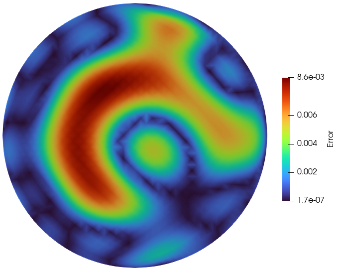
Solution Plots

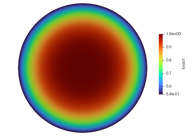
Exact Solution

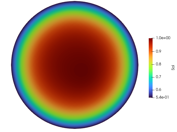
Predicted Solution

Back to Contents

References

1. FastVPINNs: Tensor-Driven Acceleration of VPINNs for Complex Geometries.

Back to Contents