Solving Inverse Problems with FastVPINNs : Estimation of spatially varying parameter on a complex geometry.
In this example, we will learn how to solve inverse problems on a complex geometry using FastVPINNs. In particular, we will solve the 2-dimensional convection-diffusion equation, as shown below, while simultaneously estimating the spatially dependent diffusion parameter \(\epsilon(x,y)\) using synthetically generated sensor data.
where
We begin by introducing the various files required to run this example
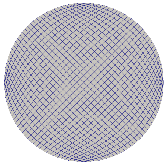
Computational Domain
The computational domain is a circular domain with radius 1 centered at (0, 0).
Contents
Steps to run the code
To run the code, execute the following command:
python3 main_inverse_domain_circle.py input_inverse_domain.yaml
Example File
The example file, cd2d_inverse_circle_example.py, defines the
boundary conditions and boundary values, the forcing function and exact
function (if test error needs to be calculated), bilinear parameters and
the actual value of the parameter that needs to be estimated (if the
error between the actual and estimated parameter needs to be calculated)
Defining the boundary values
The current version of FastVPINNs only implements Dirichlet boundary conditions. The boundary values can be set by defining a function for each boundary,
def circle_boundary(x, y):
    """
    This function will return the boundary value for given component of a boundary
    """
    val = np.ones_like(x) * 0.0
    return val
The function circle_boundary returns the boundary value for a given
component of the boundary. The function get_boundary_function_dict
returns a dictionary of boundary functions. The key of the dictionary is
the boundary id and the value is the boundary function. The function
get_bound_cond_dict returns a dictionary of boundary conditions.
def get_boundary_function_dict():
"""
This function will return a dictionary of boundary functions
"""
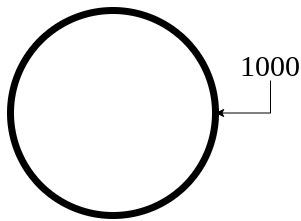
return {1000: circle_boundary}
For externally created geometries from gmsh, the user needs to provide the physical tag for the boundaries present in the geometry. In our case, we have used 1000 to define the circular boundary in mesh file.
Defining the boundary conditions
As explained above, each boundary has an identifier. The function
get_bound_cond_dict maps the boundary identifier to the boundary
condition (only Dirichlet boundary condition is implemented at this
point).
def get_bound_cond_dict():
    """
    This function will return a dictionary of boundary conditions
    """
    return {1000: circle_boundary}
Defining the forcing function
rhs can be used to define the forcing function \(f\).
def rhs(x, y):
    """
    This function will return the value of the rhs at a given point
    """
    return 10.0 * np.ones_like(x)
Defining the bilinear parameters
The bilinear parameters like diffusion constant and convective velocity
can be defined by get_bilinear_params_dict
def get_bilinear_params_dict():
    """
    This function will return a dictionary of bilinear parameters
    """

    eps = 0.1  # will not be used in the loss function, as it will be replaced by the predicted value of NN
    b1 = 1
    b2 = 0
    c = 0.0

    return {"eps": eps, "b_x": b1, "b_y": b2, "c": c}
Here, eps denoted the diffusion constant, b_x and b_y denote
the convective velocity in x and y direction respectively, and c
denotes the reaction term. In this particular example, eps is not
used in the loss calculation since it is the parameter to be estimated
and c is zero since this is simply a convection-diffusion problem.
Defining the target parameter values for testing
To test if our solver converges to the correct value of the parameter to
be estimated, we use the function get_inverse_params_actual_dict.
def get_inverse_params_actual_dict(x, y):
    """
    This function will return a dictionary of inverse parameters
    """
    # Initial Guess
    eps = 0.5 * (np.sin(x) + np.cos(y))
    return {"eps": eps}
This can then be used to calculate some error metric that assesses the performance of our solver.
Input file
The input file, input_inverse_domain.yaml, is used to define inputs
to your solver. These will usually parameters that will changed often
throughout your experimentation, hence it is best practice to pass these
parameters externally. The input file is divided based on the modules
Experimentation parameters
Defines the output path where the results will be saved.
experimentation:
  output_path: "output/inverse/circle_1"  # Path to the output directory where the results will be saved.
Geometry parameters
This section defines the geometrical parameters for your domain.
In this example, we set the
mesh_generation_methodas"external"since we want to read the mesh file for the circular domain,circular_quad.mesh.For the purposes of this example, the parameters in
internal_mesh_paramscan be ignored as they are used exclusively for internal meshes.mesh_type: FastVPINNs currently provides support for quadrilateral elements only.external_mesh_paramscan be used to specify parameters for the external mesh.mesh_file_nametakes a string (circular_quad_meshin this case).boundary_refinement_levelcontrols how many times the boundaries are refined and in effect decides the number of boundary points sampled.This sampling can be set to
uniformfor uniform sampling.
geometry:
   mesh_generation_method: "external"
   internal_mesh_params:
      x_min: 0
      x_max: 1
      y_min: 0
      y_max: 1
      n_cells_x: 20
      n_cells_y: 20
      n_boundary_points: 1500
      n_test_points_x: 100
      n_test_points_y: 100

   mesh_type: "quadrilateral"
   external_mesh_params:
      mesh_file_name: "circle_quad.mesh"  # should be a .mesh file
      boundary_refinement_level: 2
      boundary_sampling_method: "uniform"  # "uniform"
Finite element space parameters
The parameters related to the finite element space are defined here.
fe_ordersets the order of the finite element test functions.fe_typeset which type of polynomial will be used as the finite element test function.quad_orderis the number of quadrature in each direction in each cell. Thus the total number of quadrature points in each cell will be (quad_order)\(^2\).quad_typespecifies the quadrature rule to be used.
fe:
   fe_order: 3
   fe_type: "jacobi"   #"jacobi"
   quad_order:  5
   quad_type: "gauss-jacobi"  # "gauss-jacobi,
PDE beta parameters
beta specifies the weight by which the boundary loss will be
multiplied before being added to the PDE loss.
pde:
  beta: 10  # Parameter for the PDE.
Model parameters
The parameters pertaining to the neural network are specified here.
model_architectureis used to specify the dimensions of the neural network. In this example, [2, 30, 30, 30, 1] corresponds to a neural network with 2 inputs (for a 2-dimensional problem), 1 output (for a scalar problem) and 3 hidden layers with 30 neurons each.activationspecifies the activation function to be used.use_attentionspecifies if attention layers are to be used in the model. This feature is currently under development and hence should be set tofalsefor now.epochsis the number of iterations for which the network must be trained.dtypespecifies which datatype (float32orfloat64) will be used for the tensor calculations.set_memory_growth, when set toTruewill enable tensorflow’s memory growth function, restricting the memory usage on the GPU. This is currently under development and must be set toFalsefor now.learning_ratesets the learning rateinitial_learning_rateif a constant learning rate is used.A learning rate scheduler can be used by toggling
use_lr_schedulerto True and setting the corresponding decay parameters below it. Thedecay_stepsparameter is the number of steps between each learning rate decay. Thedecay_rateparameter is the decay rate for the learning rate. Thestaircaseparameter is a flag indicating whether to use the staircase decay.
model:
   model_architecture: [2, 30,30,30, 2] # output is made as 2 to accomodate the inverse param in the output
   activation: "tanh"
   use_attention: False
   epochs: 50000
   dtype: "float32"
   set_memory_growth: True
   learning_rate:
      initial_learning_rate: 0.003
      use_lr_scheduler: False
      decay_steps: 1000
      decay_rate: 0.98
      staircase: True
Logging parameters
It specifies the frequency with which the progress bar and console output will be updated, and at what interval will inference be carried out to print the solution image in the output folder.
logging:
  update_console_output: 500  # Number of steps between each update of the console output.
Inverse
Specific inputs only for inverse problems. num_sensor_points
specifies the number of points in the domain at which the solution is
known (or “sensed”). This sensor data can be synthetic or be read from a
file given by sensor_data_file.
inverse:
   num_sensor_points: 500
   sensor_data_file: "fem_output_circle2.csv"
Main file
This is the main file which needs to be run for the experiment, with the
input file as an argument. For the example, we will use the main file
main_inverse_domain_circle.py
Following are the key components of a FastVPINNs main file
Import relevant FastVPINNs methods
from fastvpinns.data.datahandler2d import DataHandler2D
from fastvpinns.FE.fespace2d import Fespace2D
from fastvpinns.Geometry.geometry_2d import Geometry_2D
Will import the functions related to setting up the finite element space, 2D Geometry and the datahandler required to manage data and make it available to the model.
from fastvpinns.model.model_inverse_domain import DenseModel_Inverse_Domain
Will import the model file where the neural network and its training
function is defined. The model file model_inverse_domain.py contains
the DenseModel_Inverse_Domain class specifically designed for
inverse problems where a spatially varying parameter has to be estimated
along with the solution.
from fastvpinns.physics.cd2d_inverse_domain import *
Will import the loss function specifically designed for this problem, with a sensor loss added to the PDE and boundary losses.
from fastvpinns.utils.compute_utils import compute_errors_combined
from fastvpinns.utils.plot_utils import plot_contour, plot_loss_function, plot_test_loss_function
from fastvpinns.utils.print_utils import print_table
Will import functions to calculate the loss, plot the results and print outputs to the console.
Reading the Input File
The input file is loaded into config and the input parameters are
read and assigned to their respective variables.
Setting up the Geometry2D object
domain = Geometry_2D(i_mesh_type, i_mesh_generation_method, i_n_test_points_x, i_n_test_points_y, i_output_path)
will instantiate a Geometry_2D object, domain, with the mesh
type, mesh generation method and test points. In our example, the mesh
generation method is external, so the cells and boundary points will
be obtained using the read_mesh method.
cells, boundary_points = domain.read_mesh(mesh_file=i_mesh_file_name, boundary_point_refinement_level=i_boundary_refinement_level,
            bd_sampling_method=i_boundary_sampling_method,
            refinement_level=0)
Reading the boundary conditions and values
As explained in the example file section, the boundary conditions and values are read as a dictionary from the example file
bound_function_dict, bound_condition_dict = get_boundary_function_dict(), get_bound_cond_dict()
Setting up the finite element space
fespace = Fespace2D(
    mesh=domain.mesh,
    cells=cells,
    boundary_points=boundary_points,
    cell_type=domain.mesh_type,
    fe_order=i_fe_order,
    fe_type=i_fe_type,
    quad_order=i_quad_order,
    quad_type=i_quad_type,
    fe_transformation_type="bilinear",
    bound_function_dict=bound_function_dict,
    bound_condition_dict=bound_condition_dict,
    forcing_function=rhs,
    output_path=i_output_path,
)
fespace will contain all the information about the finite element
space, including those read from the input fileInstantiating the inverse model
model = DenseModel_Inverse_Domain(
    layer_dims=i_model_architecture,
    learning_rate_dict=i_learning_rate_dict,
    params_dict=params_dict,
    loss_function=pde_loss_cd2d_inverse_domain,
    input_tensors_list=[datahandler.x_pde_list, train_dirichlet_input, train_dirichlet_output],
    orig_factor_matrices=[
        datahandler.shape_val_mat_list,
        datahandler.grad_x_mat_list,
        datahandler.grad_y_mat_list,
    ],
    force_function_list=datahandler.forcing_function_list,
    sensor_list=[points, sensor_values],
    tensor_dtype=i_dtype,
    use_attention=i_use_attention,
    activation=i_activation,
    hessian=False,
)
DenseModel_Inverse_Domain is a model written for inverse problems
with spatially varying parameter estimation. In this problem, we pass
the loss function pde_loss_cd2d_inverse_domain from the physics
file cd2d_inverse_domain.py.
Training the model
We are now ready to train the model to approximate the solution of the PDE while estimating the unknown diffusion parameter using the sensor data.
for epoch in range(num_epochs):

        # Train the model
        batch_start_time = time.time()

        loss = model.train_step(beta=beta, bilinear_params_dict=bilinear_params_dict)
        ...
Solution
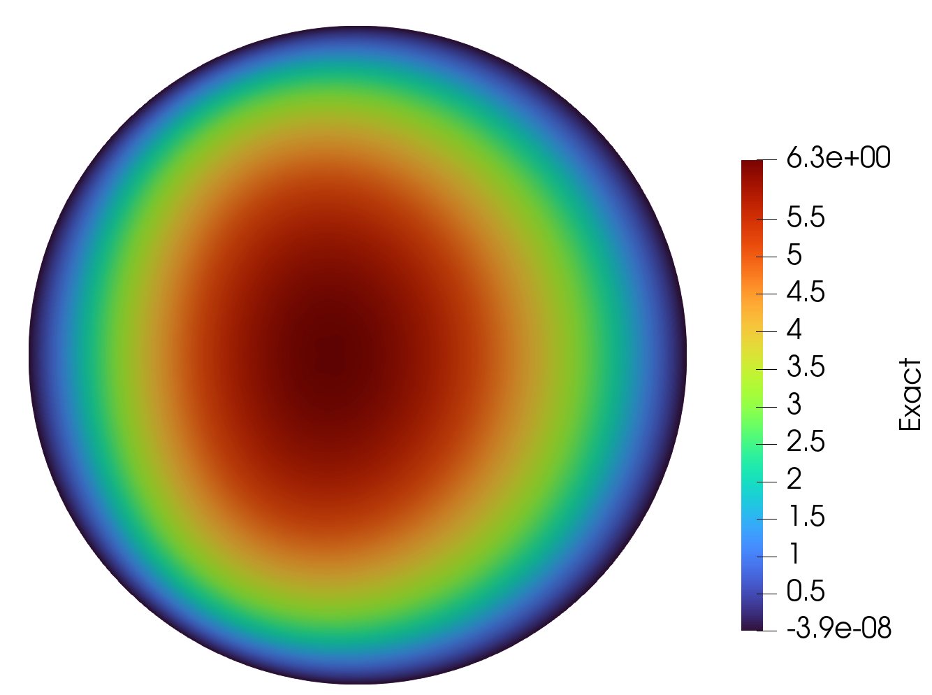
Exact Solution
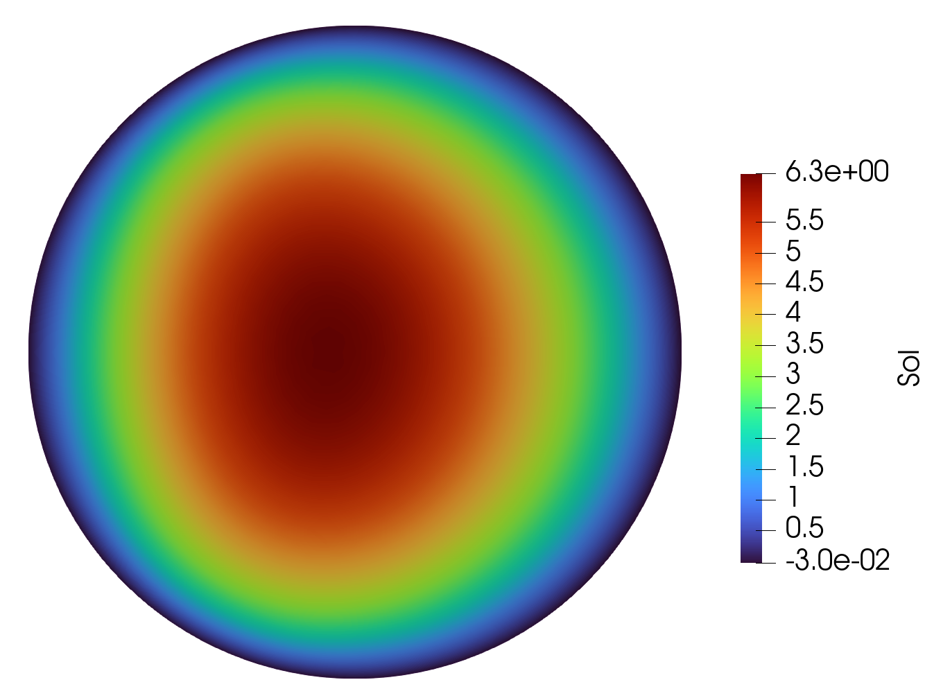
Predicted Solution
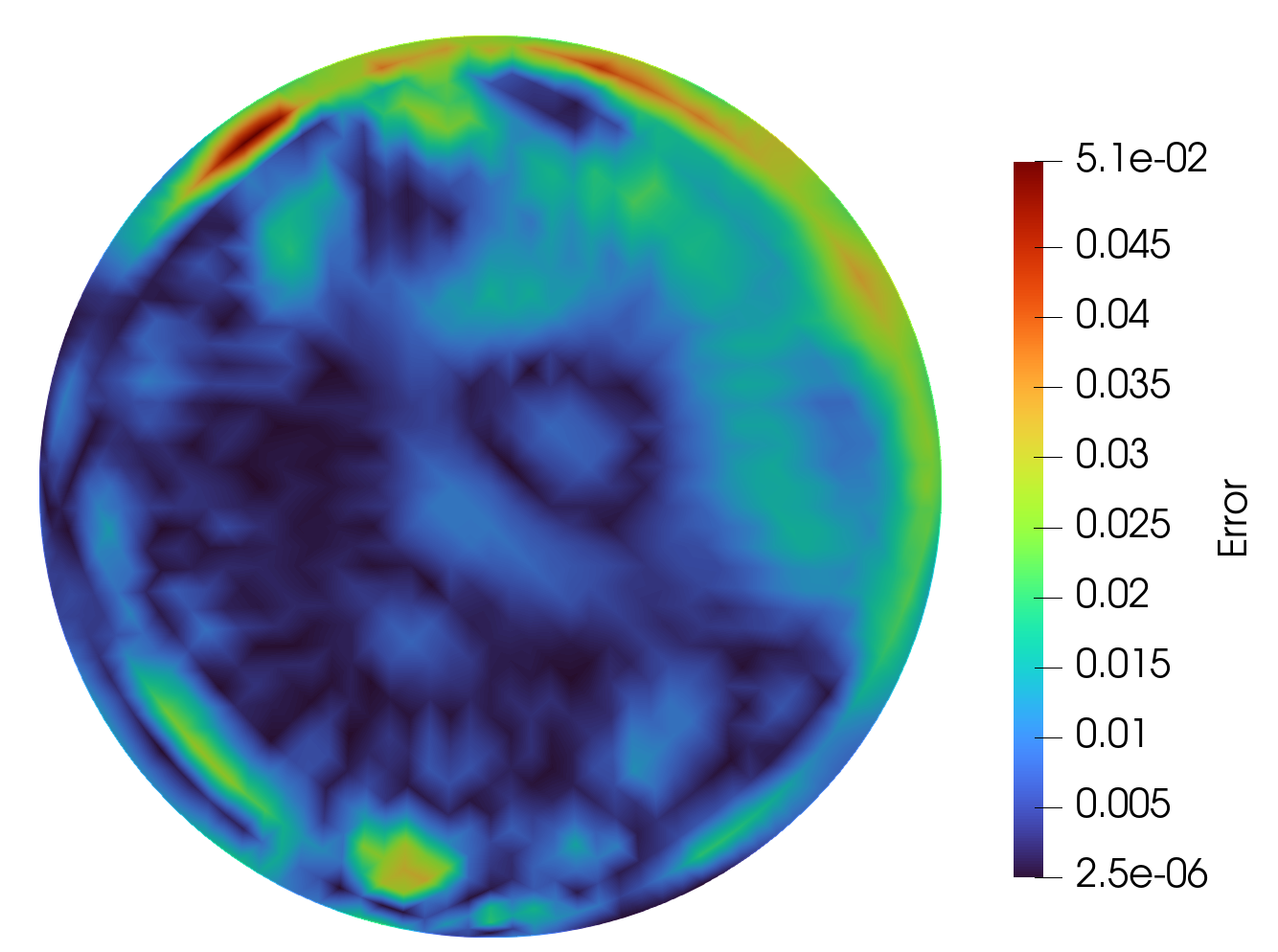
Error
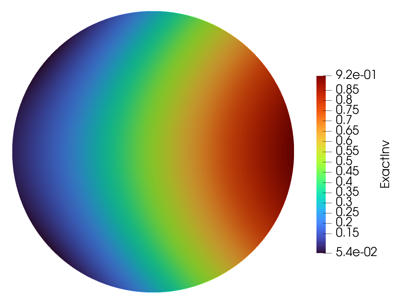
Epsilon Exact
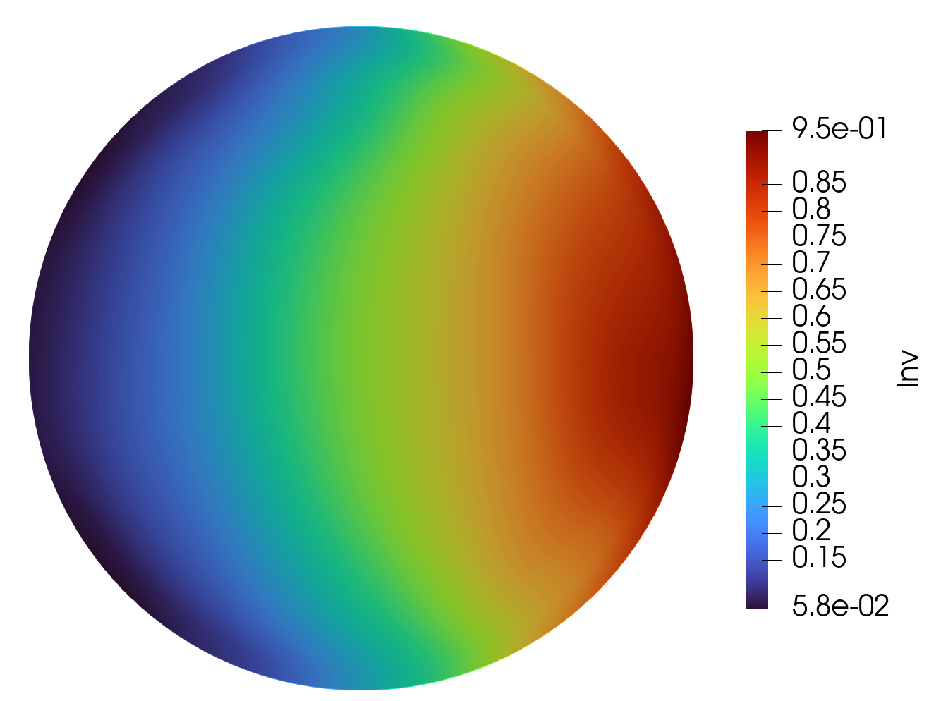
Epsilon Predicted
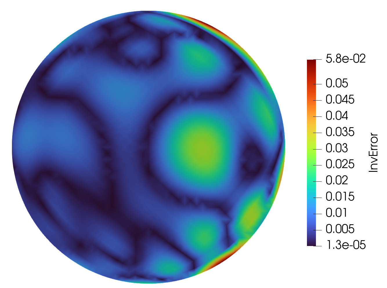
Epsilon Error